ReducedExperiment

Jack Gisby

2025-01-15

Installation

The release version of the package may be installed from Bioconductor, as follows:

if (!requireNamespace("BiocManager", quietly = TRUE)) {
    install.packages("BiocManager")
}

BiocManager::install("ReducedExperiment")

Alternatively, the development version may be installed from Bioconductor or GitHub:

BiocManager::install("ReducedExperiment", version = "devel")

devtools::install_github("jackgisby/ReducedExperiment")

Introduction

library(SummarizedExperiment)
library(ReducedExperiment)
library(ggplot2)

theme_set(theme_bw())

Dimensionality reduction approaches are often applied to reduce the complexity of high-dimensional datasets, such as gene expression data produced by microarrays and RNA sequencing. The ReducedExperiment containers are able to simultaneously store high-dimensional experimental data, sample- and feature-level metadata, and the dimensionally-reduced data.

If you are not familiar with the SummarizedExperiment containers, we suggest first reading through the package vignette, either through the Bioconductor website or by installing the package and running the following.

vignette("SummarizedExperiment", package = "SummarizedExperiment")

The key benefit of SummarizedExperiment objects is that they allow for both assay and metadata to be kept in sync while slicing and reordering the features or samples of an object. The ReducedExperiment objects inherit methods from SummarizedExperiment, so the methods available for a SummarizedExperiment object will also work on a ReducedExperiment.

When applying dimensionality reduction to high-dimensional datasets, we introduce additional complexity. In addition to assay, row and column data, we usually generate additional data matrices. For instance, methods like PCA or factor analysis tend to estimate a new matrix, with samples as rows and factors or components as columns. These methods also usually generate a loadings or rotation matrix, with features as rows and factors/components as columns.

The ReducedExperiment containers extend SummarizedExperiment by allowing for the storage and slicing of these additional matrices in tandem with our original data. This package implements ReducedExperiment, a high-level class that can store an additional matrix with samples as rows and reduced dimensions as columns. We also implemented two additional child classes for working with common dimensionality reduction methods.

The results of factor analysis can be stored in the FactorisedExperiment class, which additionally allows for the storage of a loadings matrix. The ModularExperiment class is built to store analyses based on gene modules, such as “Weighted Gene Correlation Network Analysis” (WGCNA), a popular method used to analyse transcriptomic datasets.

Relationship to existing Bioconductor packages

Several Bioconductor packages provide functionality for storing reduced dimensional representations alongside experimental data. These include packages designed for single-cell analysis, proteomics data, and other high-dimensional omics data types. These include the SingleCellExperiment Bioconductor package, which provides a reducedDims slot for storing multiple low-dimensional representations.

While there is some overlap in capabilities, ReducedExperiment serves different use cases than existing frameworks:

• Purpose: Most existing packages use dimensionality reduction primarily to enable visualisation and facilitate downstream analyses, like clustering. SingleCellExperiment, for example, is designed for single-cell workflows where reduced dimensions help manage technical noise and enable cell type identification. In contrast, ReducedExperiment focuses on methods where interpreting the components themselves is the primary goal, such as Independent Component Analysis or gene module analysis.

• Structure: While packages like SingleCellExperiment allow storage of multiple dimensionality reduction results with minimal assumptions about their generation method, ReducedExperiment implements method-specific containers (e.g., FactorisedExperiment, ModularExperiment) that enforce strict relationships between features, samples, and components to enable specialised analyses.

• Analysis Methods: ReducedExperiment provides integrated workflows for specific analysis approaches. For example, when working with ICA, it offers methods for assessing component stability and interpreting feature loadings. Some methods, like enrichment analysis, are available for multiple analysis types, with specific considerations for each.

For workflows focused primarily on visualisation, clustering, or other downstream analyses, other Bioconductor containers may be more appropriate depending on your data type and analysis goals. ReducedExperiment is best suited for analyses where the interpretation of the components themselves (such as ICA factors or gene modules) is central to the research question.

Introducing ReducedExperiment containers with a case study

There are two ways to build a ReducedExperiment object. Firstly, we provide convenience functions that both perform dimensionality reduction and package the results into the appropriate container class. We implement a method, estimateFactors, for identifying factors through Independent Component Analysis. We also provide a wrapper for applying WGCNA, identifyModules.

In this section of the vignette, we will apply both of these methods to some sample RNA sequencing data. Alternatively, if you have already applied dimensionality reduction to your data, you may simply construct a ReducedExperiment object from scratch. For instructions on how to do this, see the section entitled “Constructing a ReducedExperiment from scratch”.

The case study data

For the purposes of this vignette, we will be working with some RNA sequencing data generated for patients with COVID-19. The data were published in the following paper: https://www.nature.com/articles/s41467-022-35454-4

The data loaded below are based on the data available from the Zenodo repository: https://zenodo.org/records/6497251

The data were normalised with edgeR’s TMM method and transformed to log-counts per million. Genes with low counts were removed before further filtering to select high-variance genes. For the purposes of this example, only 500 genes were retained and we downsampled the patients.

The COVID-19 data are split up into two cohorts, one for the first wave of COVID-19 (early-mid 2020) and another for the second (early 2021). In this vignette, we will mainly use the first cohort, whereas the second cohort will be used as a validation dataset.

wave1_se <- readRDS(system.file(
    "extdata", "wave1.rds",
    package = "ReducedExperiment"
))
wave2_se <- readRDS(system.file(
    "extdata", "wave2.rds",
    package = "ReducedExperiment"
))

wave1_se

## class: SummarizedExperiment 
## dim: 500 83 
## metadata(0):
## assays(1): normal
## rownames(500): ENSG00000004799 ENSG00000007038 ... ENSG00000287935
##   ENSG00000288049
## rowData names(2): ensembl_id gene_id
## colnames(83): C37_positive_9 C48_positive_4 ... C85_negative
##   C89_negative
## colData names(8): sample_id individual_id ... case_control
##   time_from_first_x

Applying factor analysis

The first step in performing independent component analysis is to estimate the optimal number of components. We can do this with the estimateStability function. The results of this may be plotted with plotStability.

Note that this can take a long time to run. To make this faster, we could change the BPPARAM term of estimateStability to run the analysis in parallel.

The component estimation procedure is based on the maximally stable transcriptome dimension approach, described here: https://bmcgenomics.biomedcentral.com/articles/10.1186/s12864-017-4112-9

Using this method, we can plot the stability of the factors as a function of the number of components. The plot on the left shows a line for each run. We perform ICA for a sequence of components from 10 to 60, increasing the number of components by two each time. So, we run ICA for 10, 12, 14, etc. components and each of these runs produces a line in the plot. The plot on the right displays a single line displaying stability averaged over the runs.

We ideally want to pick the maximal number of components with acceptable stability. Between 30-40 components, the component stability appears to drop off, so we move forward with 35 components.

Note that the data subset we are using here has relatively few features for an RNA-seq (500). The drop-off in stability is more pronounced for the full dataset, making it easier to identify the elbow.

stability_res <- estimateStability(
    wave1_se,
    n_runs = 100,
    min_components = 10, max_components = 60, by = 2,
    mean_stability_threshold = 0.85,
    verbose = FALSE, 
    BPPARAM = BiocParallel::SerialParam(RNGseed = 1)
)

stability_plot <- plotStability(stability_res)
print(stability_plot$combined_plot)

Stability of components as a function of the number of components.

Now we run the factor analysis with these components. We additionally set a stability threshold of 0.25 to remove components with low stability. This results in the identification of 34 factors.

wave1_fe <- estimateFactors(
    wave1_se,
    nc = 35,
    use_stability = TRUE,
    n_runs = 30,
    stability_threshold = 0.25, 
    BPPARAM = BiocParallel::SerialParam(RNGseed = 1)
)

wave1_fe

## class: FactorisedExperiment 
## dim: 500 83 34 
## metadata(0):
## assays(2): normal transformed
## rownames(500): ENSG00000004799 ENSG00000007038 ... ENSG00000287935
##   ENSG00000288049
## rowData names(2): ensembl_id gene_id
## colnames(83): C37_positive_9 C48_positive_4 ... C85_negative
##   C89_negative
## colData names(8): sample_id individual_id ... case_control
##   time_from_first_x
## 34 components

The output of factor analysis is a FactorisedExperiment object. This is not dissimilar from a SummarizedExperiment object, with some additional slots. The FactorisedExperiment contains an additional matrix for the dimensionally-reduced data (i.e., samples vs. factors) and one for the factor loadings (i.e., genes vs. factors).

We can get the reduced data as so.

# get reduced data for first 5 samples and factors
reduced(wave1_fe)[1:5, 1:5]

##                   factor_1   factor_2    factor_3    factor_4   factor_5
## C37_positive_9  -1.6909747 -0.1230713 -0.64673200 -0.11119477  1.3972446
## C48_positive_4  -0.1725823 -1.3320940  0.09903561 -0.26666390  2.6840856
## C65_positive_15  1.0376609  1.3907660 -1.83762069 -0.27675565 -0.2291595
## C99_positive_13  0.8324329  0.8401592  2.16820328 -0.95320588  1.7979158
## C114_positive_9  0.8091819 -1.3398282  1.02681508  0.04833564  0.4211883

And we get the factor loadings below.

# get loadings for first 5 genes and factors
loadings(wave1_fe)[1:5, 1:5]

##                   factor_1    factor_2   factor_3    factor_4   factor_5
## ENSG00000004799 -0.7933532  0.04413147 -1.6614968 -2.67334503 -0.7278725
## ENSG00000007038 -1.2118399  0.09286032 -0.9813305 -0.62207550 -1.0048629
## ENSG00000008516  0.1902868  0.17123996 -0.2609275 -0.91819722 -0.1415753
## ENSG00000009950 -0.7733616 -0.94008770 -0.8200011 -1.56984592 -0.3755558
## ENSG00000011201 -0.6963746  0.99585966  0.8700726  0.09843149 -0.1388988

Most of the normal operations that can be performed on SummarizedExperiment objects can also be performed on FactorisedExperiments. We can slice them by samples, features and components, like so.

dim(wave1_fe[1:20, 1:10, 1:5])

##   Features    Samples Components 
##         20         10          5

Module analysis

Similarly, we can run a module analysis using the weighted gene correlation network analysis (WGCNA) package: https://bmcbioinformatics.biomedcentral.com/articles/10.1186/1471-2105-9-559

The ReducedExperiment package provides wrapper functions for running such an analysis, before packaging them into a ModularExperiment class.

First, we use the assessSoftThreshold function to determine the soft-thresholding power appropriate for our dataset. By default, the function selects the minimal power satisfying a minimal scale free topology fitting index of 0.85 and a maximal average connectivity of 100. See WGCNA’s WGCNA::pickSoftThreshold function for more details.

WGCNA::disableWGCNAThreads()

## 

wave1_fit_indices <- assessSoftThreshold(wave1_se)

wave1_estimated_power <- 
    wave1_fit_indices$Power[wave1_fit_indices$estimated_power]
print(paste0("Estimated power: ", wave1_estimated_power))

## [1] "Estimated power: 7"

Now we can pass our data with the selected power to the identifyModules function. Since for this example we’ve filtered out most of the genes that were in the original dataset, we allow for the identification of smaller modules of genes (10). The dendrogram is also stored in this object, allowing us to plot the clusters of genes that are identified.

wave1_me <- identifyModules(
    wave1_se,
    verbose = 0,
    power = wave1_estimated_power,
    minModuleSize = 10
)

plotDendro(wave1_me)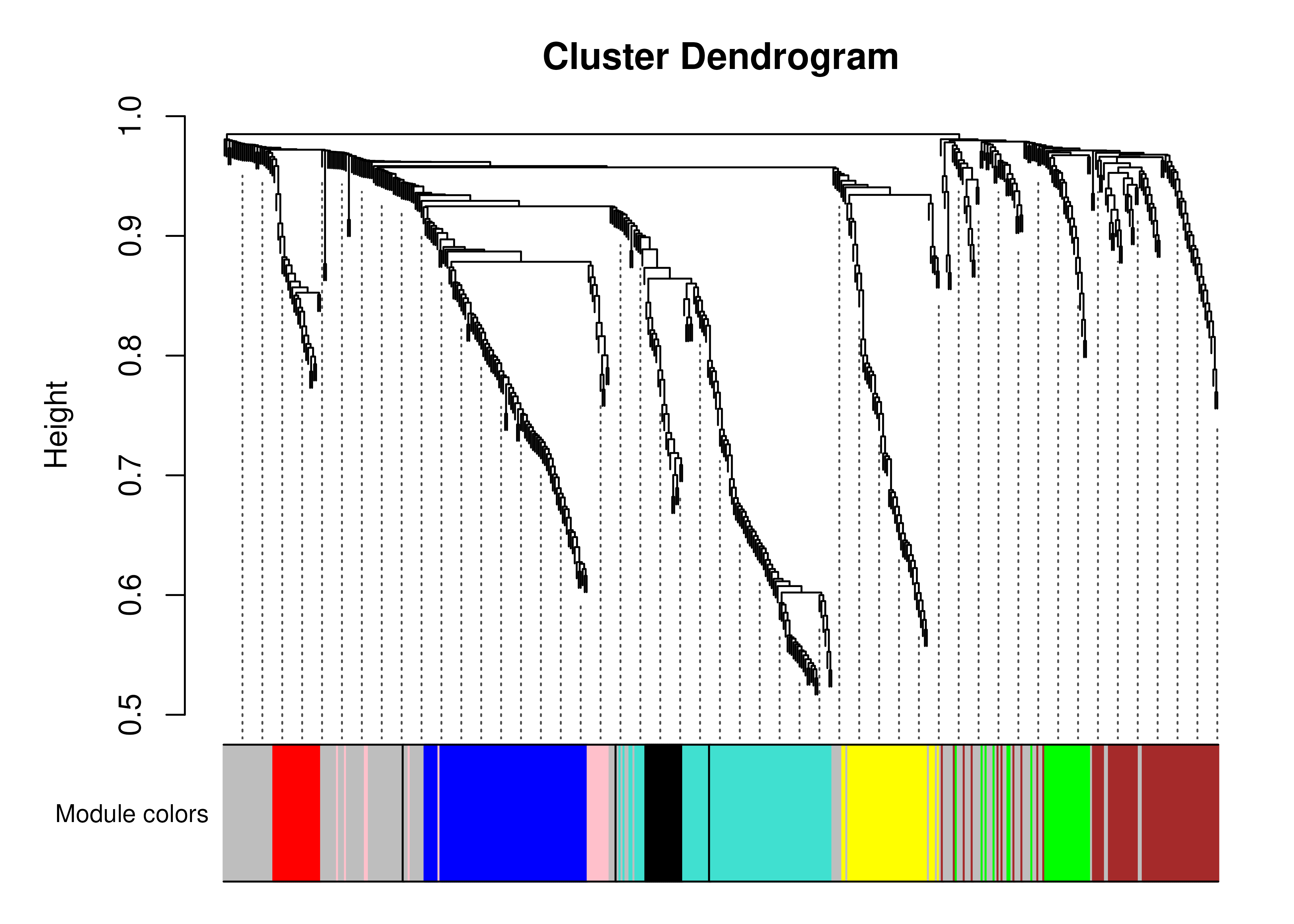

Dendrogram of the modules identified in the first wave COVID-19 data.

In this case we only identify 8 modules (module_0 is not a module itself, but rather represents the unclustered genes, and is coloured in gray in the plot above). Far more modules were identified in the original paper: https://www.nature.com/articles/s41467-022-35454-4#Fig4

This is likely because we are only using a subset of samples and genes, and we’ve used a different soft thresholding power. While identifyModules can suggest a soft thresholding power automatically, it is generally recommended that the user carefully consider the parameters used to generate modules (e.g., by considering the output of WGCNA::pickSoftThreshold). For now, however, we will move forward with our 8 modules.

wave1_me

## class: ModularExperiment 
## dim: 500 83 9 
## metadata(0):
## assays(2): normal transformed
## rownames(500): ENSG00000004799 ENSG00000007038 ... ENSG00000287935
##   ENSG00000288049
## rowData names(2): ensembl_id gene_id
## colnames(83): C37_positive_9 C48_positive_4 ... C85_negative
##   C89_negative
## colData names(8): sample_id individual_id ... case_control
##   time_from_first_x
## 9 components

The ModularExperiment functions much like a FactorisedExperiment, with a slot for the dimensionally-reduced data (samples vs. modules) and loadings (a vector containing a value for each gene). There is additionally a slot for the module assignments.

The reduced data contain expression profiles for each module that are representative of the member genes, also referred to as an “eigengene”. We can get these data as in the following chunk.

# get reduced data for first 5 samples and factors
reduced(wave1_me)[1:5, 1:5]

##                   module_0   module_1    module_2    module_3   module_4
## C37_positive_9  -0.8016005  1.7377048  2.67469604 -2.14688522 -0.5620659
## C48_positive_4   0.2296873 -0.1086692  1.45558304 -0.71718161 -0.4690700
## C65_positive_15  0.5254068  2.4265415  0.23275233 -0.83350185  0.3359459
## C99_positive_13  0.6162495  1.3848799  1.48086648 -0.70753542  2.2728971
## C114_positive_9 -0.3227018  0.3288534 -0.04067708 -0.02345718 -0.3241905

We can also find out which module each feature is assigned to.

# get assignments for first 5 genes
assignments(wave1_me)[1:5]

##          module_0          module_5          module_2          module_4 
## "ENSG00000004799" "ENSG00000007038" "ENSG00000008516" "ENSG00000009950" 
##          module_0 
## "ENSG00000011201"

The ModularExperiment object also stores the loadings, indicating the alignment of each feature with the corresponding eigengene.

# get loadings for first 5 genes
loadings(wave1_me)[1:5]

## ENSG00000004799 ENSG00000007038 ENSG00000008516 ENSG00000009950 ENSG00000011201 
##     -0.10868517      0.11835410      0.14225585      0.05915689     -0.03604060

Identifying factor and module associations

One thing we might be interested in doing is identifying factors that are associated with disease outcomes. We can do this with the associateComponents function. First, we can look at the sample-level data available in the SummarizedExperiment container.

selected_cols <- c(
    "sample_id", 
    "individual_id", 
    "case_control", 
    "sex", 
    "calc_age"
)

colData(wave1_se)[, selected_cols]

## DataFrame with 83 rows and 5 columns
##                       sample_id individual_id case_control         sex
##                     <character>   <character>  <character> <character>
## C37_positive_9   C37_positive_9           C37     POSITIVE           F
## C48_positive_4   C48_positive_4           C48     POSITIVE           M
## C65_positive_15 C65_positive_15           C65     POSITIVE           M
## C99_positive_13 C99_positive_13           C99     POSITIVE           M
## C114_positive_9 C114_positive_9          C114     POSITIVE           M
## ...                         ...           ...          ...         ...
## C257_negative     C257_negative          C257     NEGATIVE           F
## C64_negative       C64_negative           C64     NEGATIVE           M
## C69_negative       C69_negative           C69     NEGATIVE           M
## C85_negative       C85_negative           C85     NEGATIVE           F
## C89_negative       C89_negative           C89     NEGATIVE           F
##                  calc_age
##                 <integer>
## C37_positive_9         82
## C48_positive_4         72
## C65_positive_15        73
## C99_positive_13        60
## C114_positive_9        68
## ...                   ...
## C257_negative          68
## C64_negative           61
## C69_negative           79
## C85_negative           74
## C89_negative           70

In this case, we will focus on the case_control variable, indicating whether patients are COVID-19 positive or negative. For each component, we apply linear models that are adjusted for for sex and age.

f <- "~ case_control + sex + calc_age"

associations_me <- associateComponents(wave1_me, method = "lm", formula = f)
associations_fe <- associateComponents(wave1_fe, method = "lm", formula = f)

Below is a table for the significant associations between the factors and the case_control variable, encoding COVID-19 infection status.

associations_fe$summaries[
    associations_fe$summaries$term == "case_controlPOSITIVE" &
        associations_fe$summaries$adj_pvalue < 0.05,
    c("term", "component", "estimate", "stderr", "adj_pvalue")
]

##                                                term component   estimate
## factor_4_case_controlPOSITIVE  case_controlPOSITIVE  factor_4 -0.5365225
## factor_5_case_controlPOSITIVE  case_controlPOSITIVE  factor_5  1.0142974
## factor_6_case_controlPOSITIVE  case_controlPOSITIVE  factor_6 -0.5454102
## factor_8_case_controlPOSITIVE  case_controlPOSITIVE  factor_8 -0.7450610
## factor_9_case_controlPOSITIVE  case_controlPOSITIVE  factor_9  0.9025663
## factor_10_case_controlPOSITIVE case_controlPOSITIVE factor_10  1.3293240
## factor_13_case_controlPOSITIVE case_controlPOSITIVE factor_13 -0.5888254
## factor_15_case_controlPOSITIVE case_controlPOSITIVE factor_15 -0.6457925
## factor_16_case_controlPOSITIVE case_controlPOSITIVE factor_16 -0.6304351
## factor_19_case_controlPOSITIVE case_controlPOSITIVE factor_19 -0.6170465
## factor_25_case_controlPOSITIVE case_controlPOSITIVE factor_25 -0.5326069
## factor_30_case_controlPOSITIVE case_controlPOSITIVE factor_30 -0.5939576
##                                   stderr   adj_pvalue
## factor_4_case_controlPOSITIVE  0.2173879 4.586735e-02
## factor_5_case_controlPOSITIVE  0.1932897 2.146815e-05
## factor_6_case_controlPOSITIVE  0.2155776 4.554267e-02
## factor_8_case_controlPOSITIVE  0.2078114 4.939723e-03
## factor_9_case_controlPOSITIVE  0.1992191 2.334042e-04
## factor_10_case_controlPOSITIVE 0.1665895 3.247707e-10
## factor_13_case_controlPOSITIVE 0.2137396 2.752296e-02
## factor_15_case_controlPOSITIVE 0.2132976 2.262750e-02
## factor_16_case_controlPOSITIVE 0.2143364 2.337058e-02
## factor_19_case_controlPOSITIVE 0.2126742 2.337058e-02
## factor_25_case_controlPOSITIVE 0.2167430 4.586735e-02
## factor_30_case_controlPOSITIVE 0.2153104 2.752296e-02

We can plot out these results. In the plot below, factors that are “upregulated” in COVID-19 patients are shown in red, whereas “downregulated” factors are in blue. The vertical line indicates significance (i.e., adjusted p-values less than 0.05). There are a number of factors that are significantly up- or down-regulated in COVID-19.

ggplot(
    associations_fe$summaries[
        associations_fe$summaries$term == "case_controlPOSITIVE",
    ],
    aes(-log10(adj_pvalue),
        reorder(component, -log10(adj_pvalue)),
        fill = estimate
    )
) +
    geom_point(pch = 21, size = 3) +
    xlab("-log10(adjusted p-value)") +
    ylab("Factor name (ordered by adjusted p-value)") +
    geom_vline(xintercept = -log10(0.05)) +
    scale_fill_gradient2(low = "#3A3A98", high = "#832424")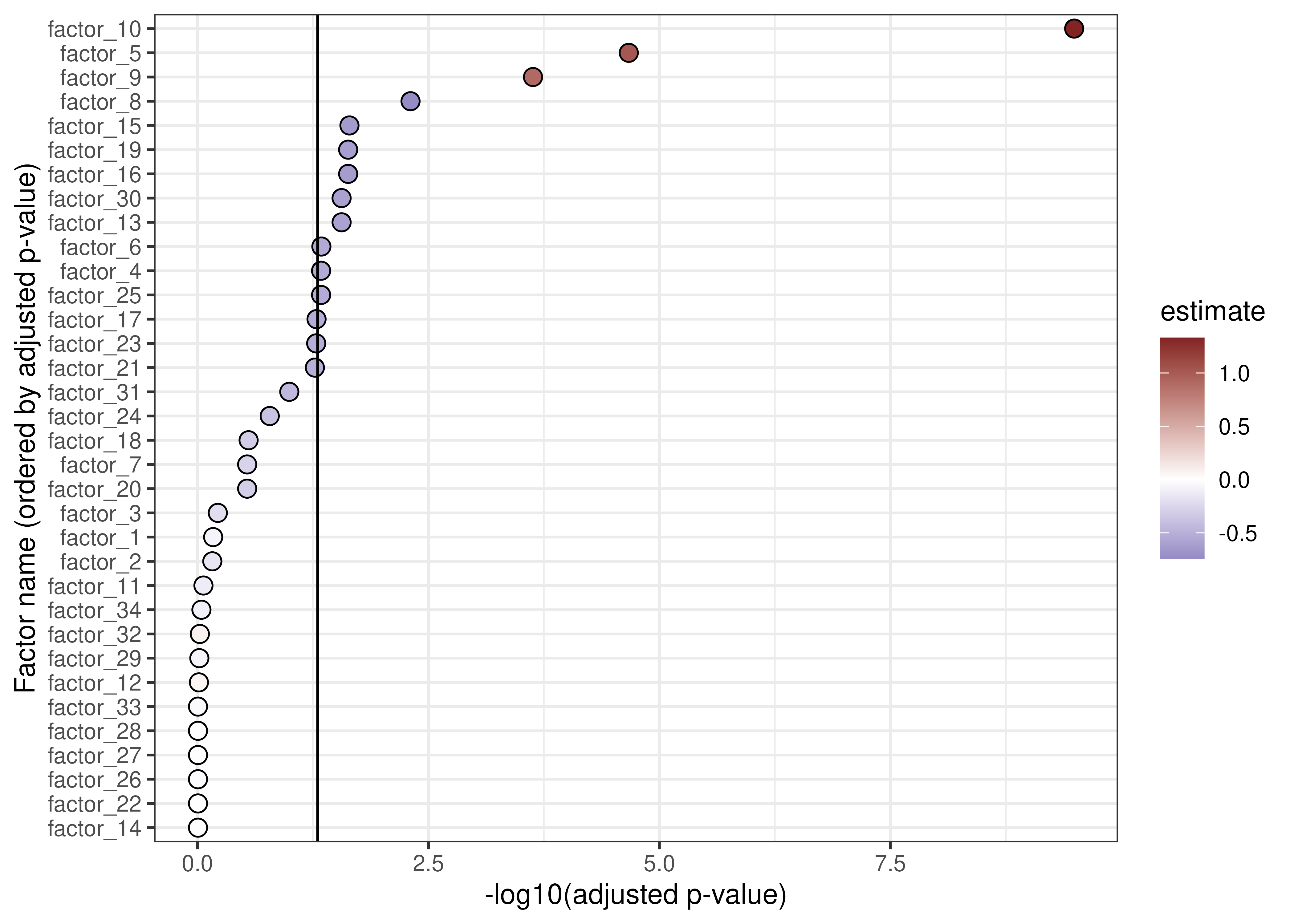

Associations between factors and COVID-19 status.

A similar plot for our modules shows significant upregulation of modules 1, 2, 7 and 8, along with down-regulation of modules 3 and 5.

ggplot(
    associations_me$summaries[
        associations_me$summaries$term == "case_controlPOSITIVE",
    ],
    aes(-log10(adj_pvalue),
        reorder(component, -log10(adj_pvalue)),
        fill = estimate
    )
) +
    geom_point(pch = 21, size = 3) +
    xlab("-log10(adjusted p-value)") +
    ylab("Module name (ordered by adjusted p-value)") +
    geom_vline(xintercept = -log10(0.05)) +
    scale_fill_gradient2(low = "#3A3A98", high = "#832424")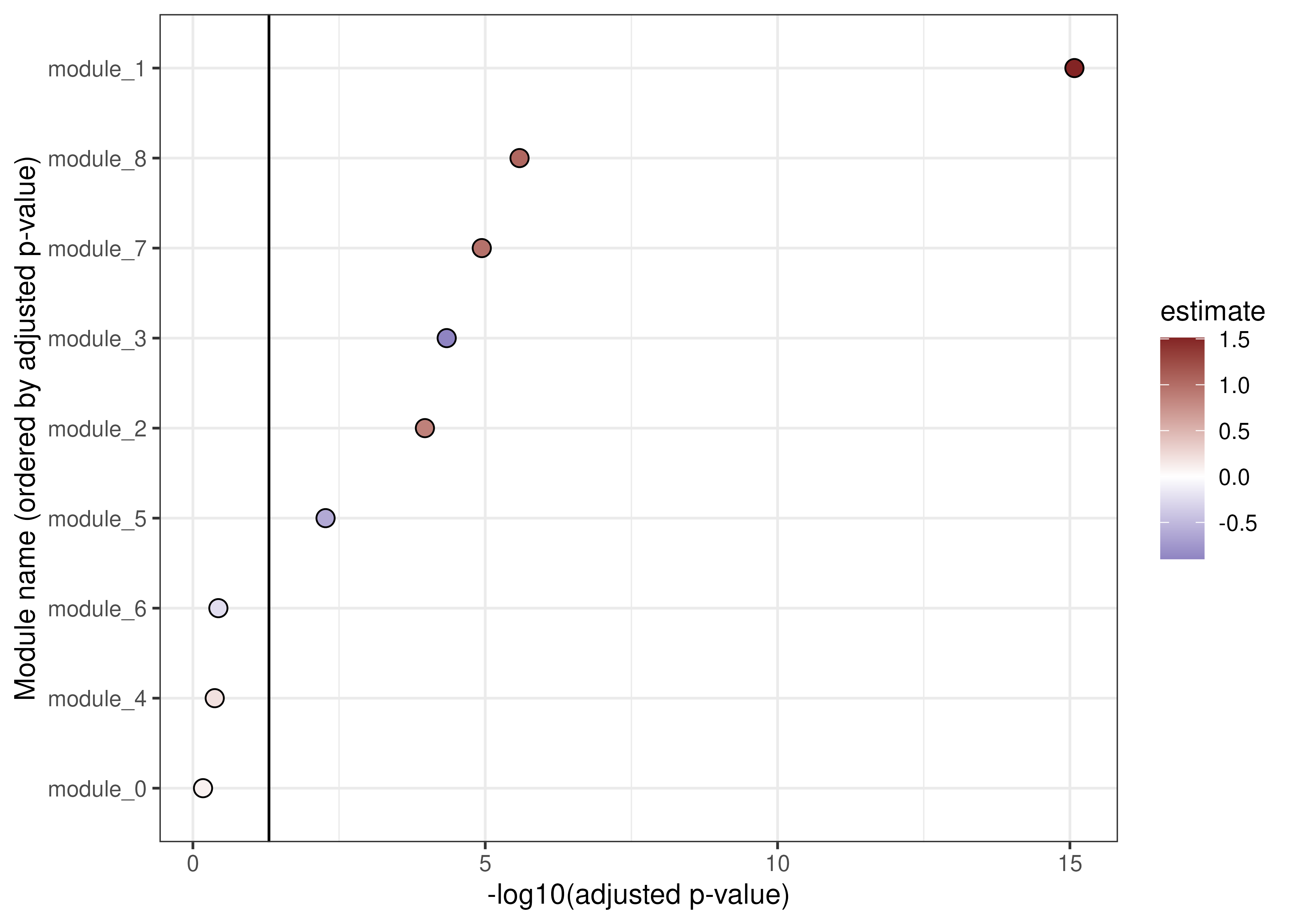

Associations between modules and COVID-19 status.

Finding functional enrichments for factors and modules

Now that we know which of our modules are up- and downregulated in COVID-19, we want to know more about the genes and pathways that are associated with our factors.

As shown before, we know which genes belong to each module by accessing the module assignments in the ModularExperiment object. We can also estimate the centrality of the genes in the module, based on the WGCNA::signedKME function.

module_centrality <- getCentrality(wave1_me)
head(module_centrality)

##       module         feature          r       rsq rank_r rank_rsq
## 125 module_0 ENSG00000286281 -0.6518679 0.4249318    128        1
## 12  module_0 ENSG00000081041 -0.6080250 0.3696945    127        2
## 37  module_0 ENSG00000151005 -0.5863308 0.3437838    126        3
## 91  module_0 ENSG00000237422  0.5792522 0.3355331      1        4
## 76  module_0 ENSG00000224020  0.5535250 0.3063899      2        5
## 126 module_0 ENSG00000286966 -0.5317176 0.2827236    125        6

This indicates the correlation of each feature with the corresponding module “eigengene”. We can also identify the genes that are highly aligned with each factor, as follows:

aligned_features <- getAlignedFeatures(wave1_fe, format = "data.frame")
head(aligned_features[, c("component", "feature", "value")])

##                 component         feature     value
## ENSG00000165246  factor_1 ENSG00000165246 11.361359
## ENSG00000288049  factor_1 ENSG00000288049  8.756050
## ENSG00000278212 factor_10 ENSG00000278212  4.413615
## ENSG00000077063 factor_10 ENSG00000077063 -3.522138
## ENSG00000204099 factor_10 ENSG00000204099  3.464273
## ENSG00000259316 factor_10 ENSG00000259316  3.096032

This shows the value of the loadings for the genes most highly associated with each factor. Some factors display moderate associations with many genes, whereas others show strong associations with just a few genes.

We can also perform pathway enrichment analyses for both factors and modules. We use the enrichment methods implemented in the clusterProfiler package. By default, these functions run gene set enrichment analysis (GSEA) and overrepresentation tests for the factors and modules, respectively. For the purposes of this vignette, we’ll just do an overrepresentation analysis for factor 5 and module 1.

TERM2GENE <- getMsigdbT2G()

factor_5_enrich <- runEnrich(
    wave1_fe[, , "factor_5"], 
    method = "overrepresentation", 
    as_dataframe = TRUE,
    TERM2GENE = TERM2GENE
)

module_1_enrich <- runEnrich(
    wave1_me[, , "module_1"], 
    method = "overrepresentation", 
    as_dataframe = TRUE,
    TERM2GENE = TERM2GENE
)

Factor 5 is enriched for the pathway “WP_NETWORK_MAP_OF_SARSCOV2_SIGNALING_PATHWAY”.

rownames(factor_5_enrich) <- NULL
factor_5_enrich[, c("ID", "pvalue", "p.adjust", "geneID")]

##                                             ID       pvalue     p.adjust
## 1 WP_NETWORK_MAP_OF_SARSCOV2_SIGNALING_PATHWAY 5.031317e-06 5.031317e-06
##                                            geneID
## 1 ENSG00000137959/ENSG00000185745/ENSG00000126709

Module 1 was upregulated in COVID-19 patients, and we see that it is primarily enriched for pathways related to complement.

ggplot(
    module_1_enrich[1:15, ],
    aes(-log10(p.adjust), reorder(substr(ID, 1, 45), -log10(p.adjust)))
) +
    geom_point(pch = 21, size = 3) +
    xlab("-log10(adjusted p-value)") +
    ylab("Pathway name (ordered by adjusted p-value)") +
    expand_limits(x = 0) +
    geom_vline(xintercept = -log10(0.05))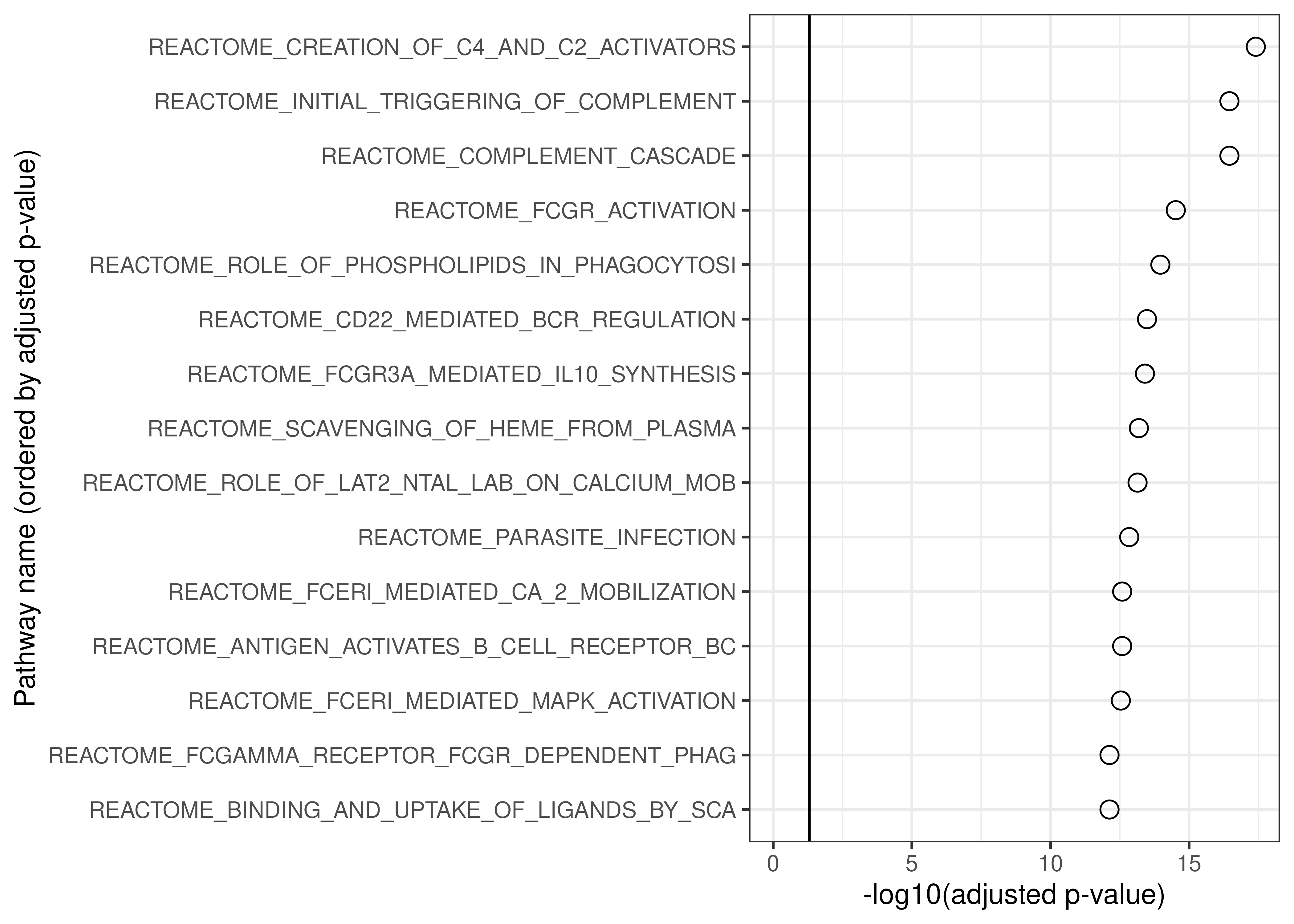

Top 15 enriched pathways for module 1.

Applying factors and modules to new datasets

Sometimes, we might want to calculate sample-level values of our factors and modules in a new dataset. In this instance, we have a second cohort that we might want to validate our results in. The ReducedExperiment package has methods for projecting new data into the factor-space defined previously and for recalculating eigengenes in new data.

Factor projection

The factor projection approach is similar to that applied by the predict method of prcomp. It uses the loadings calculated in the original dataset to calculate sample-level scores given new data. Essentially, it uses these loadings as a weighted score to perform the projection.

Doing this is very simple, as you can see below. Note, however, that these methods assume that the new data (in this case, the wave 2 data) has been processed in the same way as the original data (in this case, wave 1). By default, the method applies standardisation to the new data using the means and standard deviations calculated in the original data.

Additionally, note that, by default, the projected data are rescaled to have a mean of 0 and standard deviation of 1. So, it cannot be assumed that the projected data are on the same scale as the original data.

With all that in mind, we can apply projection as follows. These datasets were processed and normalised in the same way.

wave2_fe <- projectData(wave1_fe, wave2_se)
wave2_fe

## class: FactorisedExperiment 
## dim: 500 65 34 
## metadata(0):
## assays(1): normal
## rownames(500): ENSG00000004799 ENSG00000007038 ... ENSG00000287935
##   ENSG00000288049
## rowData names(2): ensembl_id gene_id
## colnames(65): C147_positive_11 C33_positive_11 ... C33_negative
##   C58_negative
## colData names(8): sample_id individual_id ... case_control
##   time_from_first_x
## 34 components

The new FactorisedExperiment created by projecting the wave 2 data (above) has the same genes (500) and factors (34) as the original FactorisedExperiment (below), but with different samples (83 vs. 65).

wave1_fe

## class: FactorisedExperiment 
## dim: 500 83 34 
## metadata(0):
## assays(2): normal transformed
## rownames(500): ENSG00000004799 ENSG00000007038 ... ENSG00000287935
##   ENSG00000288049
## rowData names(2): ensembl_id gene_id
## colnames(83): C37_positive_9 C48_positive_4 ... C85_negative
##   C89_negative
## colData names(8): sample_id individual_id ... case_control
##   time_from_first_x
## 34 components

While we will avoid directly comparing the dimensionally-reduced data from the two cohorts, we can calculate associations between the factors and modules and COVID-19 status, as we did in the original cohort. In this dataset there are multiple samples for each patient, so we use a linear mixed model (method = "lmer") rather than a standard linear model (method = "lm"). We also add a random intercept for the patient ID in the model formula.

replication_fe <- associateComponents(
    wave2_fe, 
    method = "lmer", 
    formula = paste0(f, " + (1|individual_id)")
)

While there are differences in the most significantly associated modules between the wave 1 and 2 cohorts, the results are broadly similar.

ggplot(
    replication_fe$summaries[
        replication_fe$summaries$term == "case_controlPOSITIVE",
    ],
    aes(
        -log10(adj_pvalue),
        reorder(component, -log10(adj_pvalue)),
        fill = estimate
    )
) +
    geom_point(pch = 21, size = 3) +
    xlab("-log10(adjusted p-value)") +
    ylab("Module name (ordered by adjusted p-value)") +
    geom_vline(xintercept = -log10(0.05)) +
    scale_fill_gradient2(low = "#3A3A98", high = "#832424") +
    expand_limits(x = 0)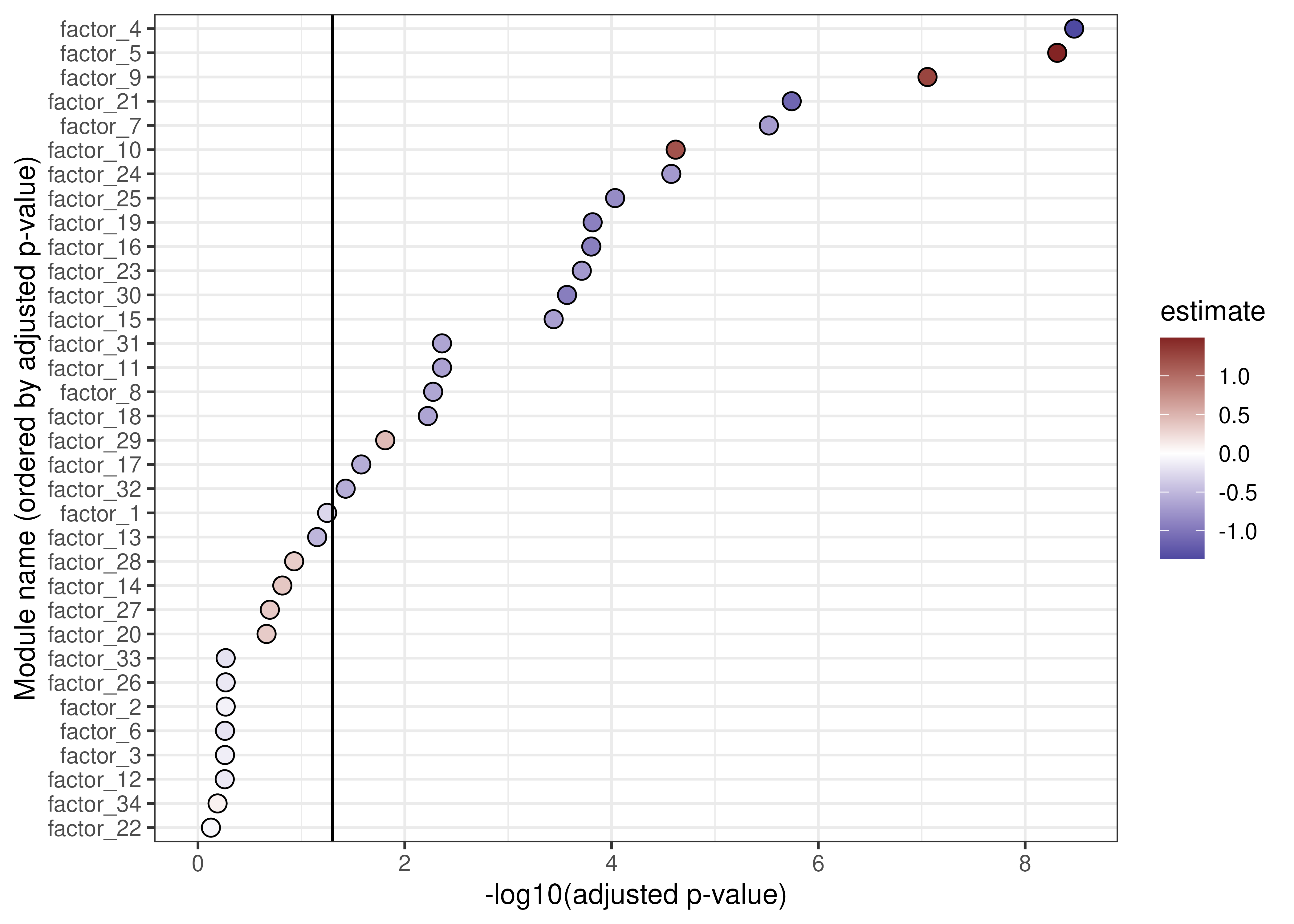

Associations between modules and COVID-19 status in the wave 2 dataset.

And, as we see in the following chunk, the estimated associations between the modules and COVID-19 status (positive vs. negative) have a strong positive correlation.

Differences in the estimated associations between modules and COVID-19 status may be explained by differences in the cohorts. For instance, different SARS-CoV-2 variants were in prevalent at the time the cohorts were sampled, and there were more treatments available for the 2021 (wave 2) cohort.

original_estimates <- associations_fe$summaries$estimate[
    associations_fe$summaries$term == "case_controlPOSITIVE"
]
replication_estimates <- replication_fe$summaries$estimate[
    replication_fe$summaries$term == "case_controlPOSITIVE"
]

cor.test(original_estimates, replication_estimates)

## 
##  Pearson's product-moment correlation
## 
## data:  original_estimates and replication_estimates
## t = 9.5767, df = 32, p-value = 6.462e-11
## alternative hypothesis: true correlation is not equal to 0
## 95 percent confidence interval:
##  0.7376086 0.9287552
## sample estimates:
##       cor 
## 0.8610094

Applying modules to new data

Similarly to factors, we can look at how our modules behave in new data. Below, we use calcEigengenes to do so, and we look at whether the modules behave similarly with respect to COVID-19 status. As we saw for factors, there is a reasonable concordance between the modules in the two datasets.

wave2_me <- calcEigengenes(wave1_me, wave2_se)

replication_me <- associateComponents(
    wave2_me, 
    method = "lmer", 
    formula = paste0(f, " + (1|individual_id)")
)

original_estimates <- associations_me$summaries$estimate[
    associations_me$summaries$term == "case_controlPOSITIVE"
]
replication_estimates <- replication_me$summaries$estimate[
    replication_me$summaries$term == "case_controlPOSITIVE"
]

cor.test(original_estimates, replication_estimates)

## 
##  Pearson's product-moment correlation
## 
## data:  original_estimates and replication_estimates
## t = 2.8828, df = 7, p-value = 0.02356
## alternative hypothesis: true correlation is not equal to 0
## 95 percent confidence interval:
##  0.1422098 0.9406294
## sample estimates:
##       cor 
## 0.7367495

Module preservation

We can also consider the preservation of modules. Below, we take our modules calculated in the Wave 1 dataset, and assess their reproducibility in the Wave 2 dataset. A variety of statistics are calculated by WGCNA’s modulePreservation. By default, the plotModulePreservation function shows us the “medianRank” and “Zsummary” statistics. You can find out more about these in the corresponding publication, but in general we are interested in modules with higher Zsummary scores. In short, we can consider modules above the blue line (Z > 2) to be moderately preserved and modules above the green line (Z > 10) to be highly preserved. We see that modules 1 and 2 have relatively high preservation in the Wave 2 dataset, whereas modules 5 and 0 (our unclustered genes) display relatively low preservation.

# Using a low number of permutations for the vignette
mod_pres_res <- modulePreservation(
    wave1_me, 
    wave2_se, 
    verbose = 0, 
    nPermutations = 5
)

plotModulePreservation(mod_pres_res)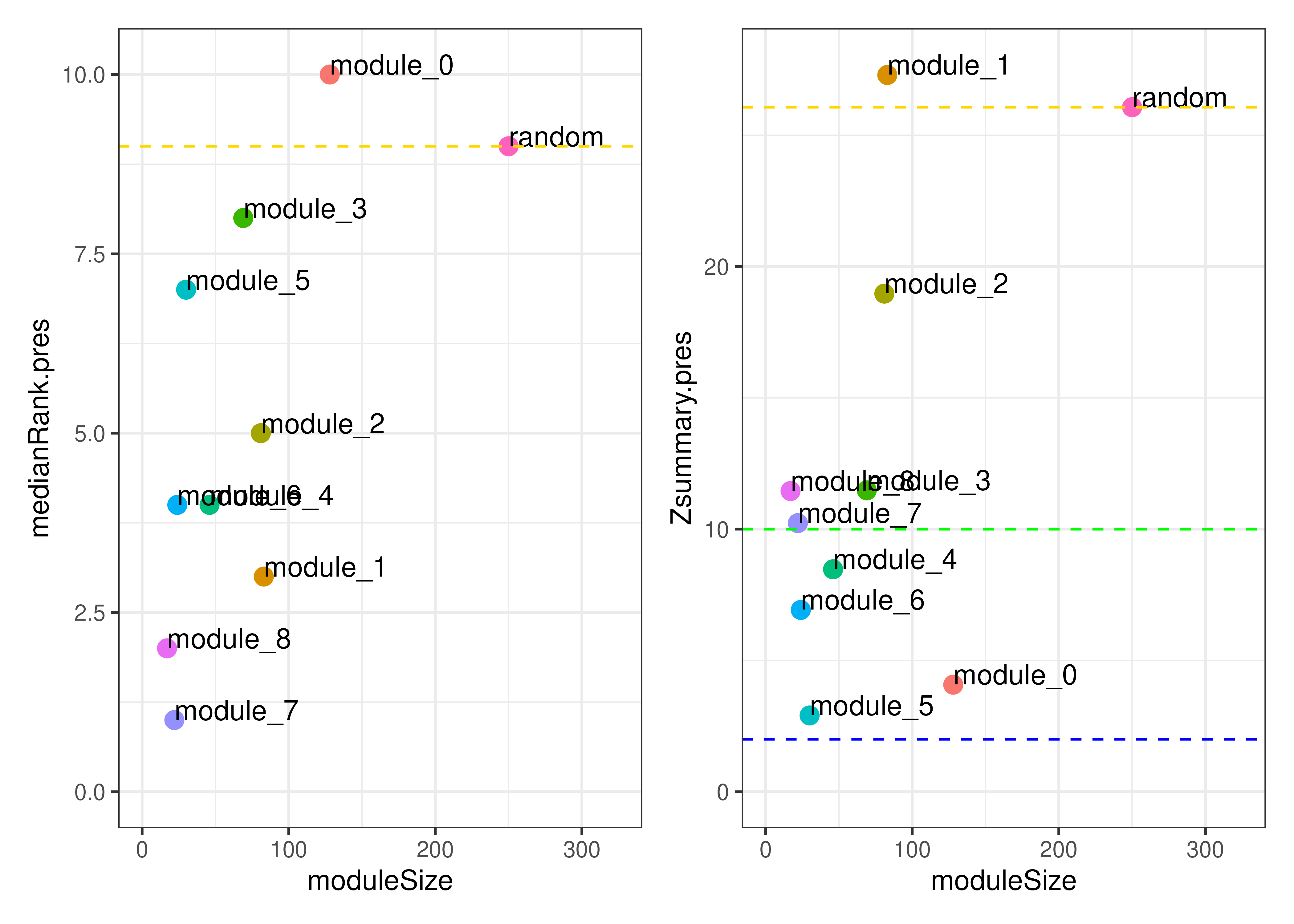

Module preservation between the Wave 1 and Wave 2 datasets.

Extending the ReducedExperiment class

The SummarizedExperiment package includes a detailed vignette explaining how to derive new containers from the SummarizedExperiment class.

vignette("Extensions", package = "SummarizedExperiment")

The ReducedExperiment containers may be extended in a similar fashion. In this package, we implemented ReducedExperiment and two derivative classes, ModularExperiment and FactorisedExperiment. While these are convenient for working with the output of module and factor analysis, respectively, other dimensionality reduction approaches may require the incorporation of additional components and methods.

For instance, we could define a PCAExperiment class for storing the output of stats::prcomp (i.e., Principal Components Analysis, or PCA). The function produces the following:

• x: The reduced data, which we will store in the existing ReducedExperiment reduced slot.
• rotation: The feature loadings, for which we will create a new slot,
• sdev: The standard deviations of the principal components, for which we will create a new slot.
• center and scale: The centering and scaling used, which we will store in their existing ReducedExperiment slots.

PCAExperiment <- setClass(
    "PCAExperiment",
    contains = "ReducedExperiment",
    slots = representation(
        rotation = "matrix",
        sdev = "numeric"
    )
)

We may then run stats::prcomp on our data and store the output in a PCAExperiment container. We give the original SummarizedExperiment object as an argument, and we also supply the outputs of stats::prcomp to the slots defined for ReducedExperiment and the new slots defined above for PCAExperiment.

prcomp_res <- stats::prcomp(t(assay(wave1_se)), center = TRUE, scale. = TRUE)

my_pca_experiment <- PCAExperiment(
    wave1_se,
    reduced = prcomp_res$x,
    rotation = prcomp_res$rotation,
    sdev = prcomp_res$sdev,
    center = prcomp_res$center,
    scale = prcomp_res$scale
)

my_pca_experiment

## class: PCAExperiment 
## dim: 500 83 83 
## metadata(0):
## assays(1): normal
## rownames(500): ENSG00000004799 ENSG00000007038 ... ENSG00000287935
##   ENSG00000288049
## rowData names(2): ensembl_id gene_id
## colnames(83): C37_positive_9 C48_positive_4 ... C85_negative
##   C89_negative
## colData names(8): sample_id individual_id ... case_control
##   time_from_first_x
## 83 components

We can retrieve the principal components.

reduced(my_pca_experiment)[1:5, 1:5]

##                        PC1        PC2       PC3       PC4        PC5
## C37_positive_9  -22.648920   2.073466 -8.868433  4.937109 -0.4326127
## C48_positive_4  -10.432551   6.505781 -7.716721 -3.955820  6.5379878
## C65_positive_15 -13.971056 -10.765106  3.059072  2.940002  2.0719260
## C99_positive_13 -18.902753   1.955157  8.360083 -6.745072  2.4953812
## C114_positive_9  -1.939066  -3.262649 -2.722028 -1.963664  6.3567510

But to retrieve our new rotation matrix we need to define a “getter” method.

setGeneric("rotation", function(x, ...) standardGeneric("rotation"))

## [1] "rotation"

setMethod("rotation", "PCAExperiment", function(x, withDimnames = TRUE) {
    return(x@rotation)
})

rotation(my_pca_experiment)[1:5, 1:5]

##                          PC1         PC2           PC3           PC4
## ENSG00000004799 -0.010245337  0.02572064  0.0393218628  5.047993e-02
## ENSG00000007038  0.026332021 -0.02255524  0.0107295922 -4.530682e-02
## ENSG00000008516 -0.070317116  0.08858630 -0.0124291253  7.538345e-05
## ENSG00000009950 -0.015691540  0.02310483  0.0511868032  1.173290e-01
## ENSG00000011201 -0.008071982  0.04992057 -0.0007111778 -8.025871e-03
##                         PC5
## ENSG00000004799  0.06974641
## ENSG00000007038 -0.06941132
## ENSG00000008516 -0.03389891
## ENSG00000009950  0.02693113
## ENSG00000011201  0.01287611

And to change the values of the rotation matrix we must also define a setter:

setGeneric("rotation<-", function(x, ..., value) standardGeneric("rotation<-"))

## [1] "rotation<-"

setReplaceMethod("rotation", "PCAExperiment", function(x, value) {
    x@rotation <- value
    validObject(x)
    return(x)
})

# Set the value at position [1, 1] to 10 and get
rotation(my_pca_experiment)[1, 1] <- 10
rotation(my_pca_experiment)[1:5, 1:5]

##                          PC1         PC2           PC3           PC4
## ENSG00000004799 10.000000000  0.02572064  0.0393218628  5.047993e-02
## ENSG00000007038  0.026332021 -0.02255524  0.0107295922 -4.530682e-02
## ENSG00000008516 -0.070317116  0.08858630 -0.0124291253  7.538345e-05
## ENSG00000009950 -0.015691540  0.02310483  0.0511868032  1.173290e-01
## ENSG00000011201 -0.008071982  0.04992057 -0.0007111778 -8.025871e-03
##                         PC5
## ENSG00000004799  0.06974641
## ENSG00000007038 -0.06941132
## ENSG00000008516 -0.03389891
## ENSG00000009950  0.02693113
## ENSG00000011201  0.01287611

To fully flesh out our class we would also need to consider:

• Defining getters and setters for the sdev slot
• Implementing a constructor method to make creating PCAExperiment simpler and add sensible defaults
• Implementing a method to check the validity of our object
• Modifying existing methods, such as subsetting operations (i.e., ]), to handle the new slots we have introduced

For the ModularExperiment and FactorisedExperiment classes, we additionally implemented a variety of methods specific to the type of data they store. Since the results of PCA are similar to that of factor analysis, in practice it would likely be more straightforward to simply store these results in a FactorisedExperiment.

Constructing a ReducedExperiment from scratch

If you have already applied dimensionality reduction to your data, you may be able to package the results into one of the ReducedExperiment containers. Below, we construct a FactorisedExperiment container based on the results of PCA applied to gene expression data. This container is appropriate, because we can store the sample-level principal components in the reduced slot of the object, and we may store the rotation matrix returned by stats::prcomp to the loadings slot.

To construct our FactorisedExperiment, we provide a SummarizedExperiment as our first argument. In this case we reconstruct our SummarizedExperiment for demonstration purposes, but if you have already constructed a SummarizedExperiment you may simply pass this as the first argument.

We then pass the results of stats::prcomp to the object’s slots. This object is now ready to work with as described in the section above (“Introducing ReducedExperiment containers with a case study”).

# Construct a SummarizedExperiment (if you don't already have one)
expr_mat <- assay(wave1_se)
pheno_data <- colData(wave1_se)
se <- SummarizedExperiment(
    assays = list("normal" = expr_mat),
    colData = pheno_data
)

# Calculate PCA with prcomp
prcomp_res <- stats::prcomp(t(assay(se)), center = TRUE, scale. = TRUE)

# Create a FactorisedExperiment container
fe <- FactorisedExperiment(
    se,
    reduced = prcomp_res$x,
    loadings = prcomp_res$rotation,
    stability = prcomp_res$sdev,
    center = prcomp_res$center,
    scale = prcomp_res$scale
)

fe

## class: FactorisedExperiment 
## dim: 500 83 83 
## metadata(0):
## assays(1): ''
## rownames(500): ENSG00000004799 ENSG00000007038 ... ENSG00000287935
##   ENSG00000288049
## rowData names(0):
## colnames(83): C37_positive_9 C48_positive_4 ... C85_negative
##   C89_negative
## colData names(0):
## 83 components

Vignette references

This vignette used publicly available gene expression data (RNA sequencing) from the following publication:

• “Multi-omics identify falling LRRC15 as a COVID-19 severity marker and persistent pro-thrombotic signals in convalescence” (https://doi.org/10.1038/s41467-022-35454-4)
  • Gisby et al., 2022
• Zenodo data deposition (https://zenodo.org/doi/10.5281/zenodo.6497250)

The stability-based ICA algorithm implemented in this package for identifying latent factors is based on the ICASSO algorithm, references for which can be found below:

• “Icasso: software for investigating the reliability of ICA estimates by clustering and visualization” (https://doi.org/10.1109/NNSP.2003.1318025)
  • Himberg et al., 2003
• “stabilized-ica” Python package (https://github.com/ncaptier/stabilized-ica)
  • Nicolas Captier

The estimateStability function is based on the related Most Stable Transcriptome Dimension approach, which also has a Python implementation provided by the stabilized-ica Python package.

• “Determining the optimal number of independent components for reproducible transcriptomic data analysis” (https://doi.org/10.1186/s12864-017-4112-9)
  • Kairov et al., 2017

Identification of coexpressed gene modules is carried out through the Weighted Gene Correlation Network Analysis (WGCNA) framework

• “WGCNA: an R package for weighted correlation network analysis” (https://doi.org/10.1186/1471-2105-9-559)
  • Langfelder and Horvath, 2008
• “WGCNA” R package (https://cran.r-project.org/web/packages/WGCNA/index.html)
• “Is My Network Module Preserved and Reproducible?” (https://doi.org/10.1371/journal.pcbi.1001057)
  • Langfelder, Luo, Oldham and Horvath, 2011

Session Information

Here is the output of sessionInfo() on the system on which this document was compiled:

## R version 4.4.2 (2024-10-31)
## Platform: x86_64-pc-linux-gnu
## Running under: Ubuntu 24.04.1 LTS
## 
## Matrix products: default
## BLAS:   /usr/lib/x86_64-linux-gnu/openblas-pthread/libblas.so.3 
## LAPACK: /usr/lib/x86_64-linux-gnu/openblas-pthread/libopenblasp-r0.3.26.so;  LAPACK version 3.12.0
## 
## locale:
##  [1] LC_CTYPE=en_US.UTF-8       LC_NUMERIC=C              
##  [3] LC_TIME=en_US.UTF-8        LC_COLLATE=en_US.UTF-8    
##  [5] LC_MONETARY=en_US.UTF-8    LC_MESSAGES=en_US.UTF-8   
##  [7] LC_PAPER=en_US.UTF-8       LC_NAME=C                 
##  [9] LC_ADDRESS=C               LC_TELEPHONE=C            
## [11] LC_MEASUREMENT=en_US.UTF-8 LC_IDENTIFICATION=C       
## 
## time zone: UTC
## tzcode source: system (glibc)
## 
## attached base packages:
## [1] stats4    stats     graphics  grDevices utils     datasets  methods  
## [8] base     
## 
## other attached packages:
##  [1] ggplot2_3.5.1               ReducedExperiment_0.99.6   
##  [3] SummarizedExperiment_1.36.0 Biobase_2.66.0             
##  [5] GenomicRanges_1.58.0        GenomeInfoDb_1.42.1        
##  [7] IRanges_2.40.1              S4Vectors_0.44.0           
##  [9] BiocGenerics_0.52.0         MatrixGenerics_1.18.1      
## [11] matrixStats_1.5.0           BiocStyle_2.34.0           
## 
## loaded via a namespace (and not attached):
##   [1] splines_4.4.2           ggplotify_0.1.2         filelock_1.0.3         
##   [4] tibble_3.2.1            R.oo_1.27.0             preprocessCore_1.68.0  
##   [7] rpart_4.1.24            lifecycle_1.0.4         httr2_1.0.7            
##  [10] Rdpack_2.6.2            fastcluster_1.2.6       doParallel_1.0.17      
##  [13] lattice_0.22-6          MASS_7.3-64             backports_1.5.0        
##  [16] magrittr_2.0.3          Hmisc_5.2-2             sass_0.4.9             
##  [19] rmarkdown_2.29          jquerylib_0.1.4         yaml_2.3.10            
##  [22] ggtangle_0.0.6          cowplot_1.1.3           DBI_1.2.3              
##  [25] minqa_1.2.8             RColorBrewer_1.1-3      abind_1.4-8            
##  [28] zlibbioc_1.52.0         purrr_1.0.2             R.utils_2.12.3         
##  [31] msigdbr_7.5.1           yulab.utils_0.1.9       nnet_7.3-20            
##  [34] rappdirs_0.3.3          GenomeInfoDbData_1.2.13 enrichplot_1.26.6      
##  [37] ggrepel_0.9.6           tidytree_0.4.6          moments_0.14.1         
##  [40] pkgdown_2.1.1           codetools_0.2-20        DelayedArray_0.32.0    
##  [43] DOSE_4.0.0              xml2_1.3.6              tidyselect_1.2.1       
##  [46] aplot_0.2.4             UCSC.utils_1.2.0        farver_2.1.2           
##  [49] lme4_1.1-36             BiocFileCache_2.14.0    dynamicTreeCut_1.63-1  
##  [52] base64enc_0.1-3         jsonlite_1.8.9          Formula_1.2-5          
##  [55] survival_3.8-3          iterators_1.0.14        systemfonts_1.1.0      
##  [58] foreach_1.5.2           tools_4.4.2             progress_1.2.3         
##  [61] treeio_1.30.0           ragg_1.3.3              ica_1.0-3              
##  [64] Rcpp_1.0.14             glue_1.8.0              gridExtra_2.3          
##  [67] SparseArray_1.6.0       xfun_0.50               qvalue_2.38.0          
##  [70] dplyr_1.1.4             withr_3.0.2             numDeriv_2016.8-1.1    
##  [73] BiocManager_1.30.25     fastmap_1.2.0           boot_1.3-31            
##  [76] digest_0.6.37           R6_2.5.1                gridGraphics_0.5-1     
##  [79] textshaping_0.4.1       colorspace_2.1-1        GO.db_3.20.0           
##  [82] biomaRt_2.62.0          RSQLite_2.3.9           R.methodsS3_1.8.2      
##  [85] tidyr_1.3.1             generics_0.1.3          data.table_1.16.4      
##  [88] prettyunits_1.2.0       httr_1.4.7              htmlwidgets_1.6.4      
##  [91] S4Arrays_1.6.0          pkgconfig_2.0.3         gtable_0.3.6           
##  [94] blob_1.2.4              impute_1.80.0           XVector_0.46.0         
##  [97] clusterProfiler_4.14.4  htmltools_0.5.8.1       carData_3.0-5          
## [100] bookdown_0.42           fgsea_1.32.2            scales_1.3.0           
## [103] png_0.1-8               reformulas_0.4.0        ggfun_0.1.8            
## [106] knitr_1.49              rstudioapi_0.17.1       reshape2_1.4.4         
## [109] checkmate_2.3.2         nlme_3.1-166            curl_6.1.0             
## [112] nloptr_2.1.1            cachem_1.1.0            stringr_1.5.1          
## [115] parallel_4.4.2          foreign_0.8-88          AnnotationDbi_1.68.0   
## [118] desc_1.4.3              pillar_1.10.1           grid_4.4.2             
## [121] vctrs_0.6.5             car_3.1-3               dbplyr_2.5.0           
## [124] cluster_2.1.8           htmlTable_2.4.3         evaluate_1.0.3         
## [127] cli_3.6.3               compiler_4.4.2          rlang_1.1.4            
## [130] crayon_1.5.3            labeling_0.4.3          plyr_1.8.9             
## [133] fs_1.6.5                stringi_1.8.4           WGCNA_1.73             
## [136] BiocParallel_1.40.0     babelgene_22.9          lmerTest_3.1-3         
## [139] munsell_0.5.1           Biostrings_2.74.1       lazyeval_0.2.2         
## [142] GOSemSim_2.32.0         Matrix_1.7-1            hms_1.1.3              
## [145] patchwork_1.3.0         bit64_4.5.2             KEGGREST_1.46.0        
## [148] rbibutils_2.3           igraph_2.1.3            memoise_2.0.1          
## [151] bslib_0.8.0             ggtree_3.14.0           fastmatch_1.1-6        
## [154] bit_4.5.0.1             gson_0.1.0              ape_5.8-1